From Ink Drops to Light Loops: Solving Physics at the Speed of Light

Imagine a single drop of ink falling into a clear cup of water. Right after the drop hits the surface, the ink is highly concentrated in one spot. As time goes on, the stain spreads out. The density of ink at any point in the cup depends on two things: how much ink was there a moment ago, and how much ink sits in the neighboring regions. The mathematical description of such a process, among many other physical processes, is given by a partial differential equation (PDE).

For a few idealized situations, such equations could be solved analytically. In most situations, however, the dynamics must be solved numerically. Consider a PDE of the type $\frac{dU}{dt}=O(U),$ where $U$ describes for instance the ink concentration. To know the ink distribution at some time $t_1$ we must take our initial conditions at time $t_0$ , apply the operator $O$ , and get the distribution at time $t_0+dt$. And then again. And again. A PDE solver is essentially a very fast machine for repeating this process on a very large grid.

On a digital processor, this is hard work. The grid can easily have millions of points, and at each time step the processor must move data back and forth to memory, compute interactions with neighbours, and store the updated values. As the physics becomes more complex – each point “talks” to more neighbours, or the operator has more terms – the amount of data movement grows. Sooner or later moving bits between memory and processor becomes a serious bottleneck. Could we do something differently?

The Light-Speed Optical Loop

In LightSolver’s Laser Processing Unit™ (LPU), the story is indeed very different. The state of the PDE is not stored in RAM. Instead, it is stored in the phase of a light field, circulating inside a programmable optical resonator. Each point on the PDE domain’s grid corresponds to a point in the transverse profile of the beam. Each time the light completes a round trip, it passes through a sequence of optical elements that act as the operator $O$.

Crucially, the duration of that step is set by the cavity round-trip time, which is on the order of a few nanoseconds. This “clock cycle” does not grow with problem size or connectivity. Whether the operator couples each point only to its four nearest neighbours or to a more intricate web of interactions across the whole image, the light still traverses the same optical path in the same amount of time, and all grid points are updated in parallel. Complexity may, however, influence how many iterations you need to reach a solution.

The Challenges – Survival and Boundaries

This elegant picture conceals two important constraints: The first is the steady-state problem. If the cup is left on the table for long enough, the ink stops changing, and it reaches a steady state. At that point $\frac{dU}{dt}=0$ , which means $O(U)=0$ . In many engineering problems, this steady state is exactly what you want – the final temperature map, the electrostatic potential, the pressure distribution once everything has settled.

But here’s the catch: If we built a simple laser cavity where the optical operator directly defines the field update, then as the system approaches the solution and the change tends to zero, the operator would effectively stop feeding light back into the cavity. From the laser’s point of view, a result of “zero” looks like “no light”. The gain medium no longer has anything to amplify, the field decays below threshold, and the very solution we have just converged to disappears. The computation would literally turn off its own light.

The second constraint is boundaries. The ink-in-water picture hides another essential ingredient: the cup itself. As the ink spreads, it eventually reaches the wall. What happens there? Does the concentration stick to a fixed value at the glass? Can ink leak out? Mathematically, these are boundary conditions, and they are an important part of defining the PDE. Any practical solver must encode them too.

The Split-Loop Solution

These dual challenges – maintaining the solution at steady state while respecting boundary constraints – motivate our split-loop architecture. We divide the cavity into two logical parts: a memory loop and an operator loop.

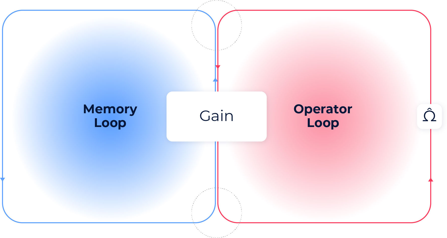
The memory loop is responsible for keeping the laser alive and stable, independent of what the PDE is doing. It ensures that even when $O(U)=0$ , the light field persists, carrying the converged solution without fading away.

The operator loop is where the evolution happens. A controlled fraction of the light is peeled off, sent through the optical elements that implement the physics and boundary conditions, and then reinjected to gently update the phase of the main beam. This separation allows the system to converge to steady state without extinguishing itself, while simultaneously enforcing the geometric and physical constraints of the problem.

In the next post, we will pop the hood on this split-loop architecture and show how lenses, beam splitters, spatial light modulators and a digital micromirror device physically encode the mathematical operations.

If you are interested and want to hear more, you are welcome to check out our paper, demonstrating our approach to solving PDEs, or contact us so we could discuss how LightSolver’s LPU could help solve your PDEs.